Raising e to a Matrix, and Why Schrödinger's Equation Is a Rotation

August 2026

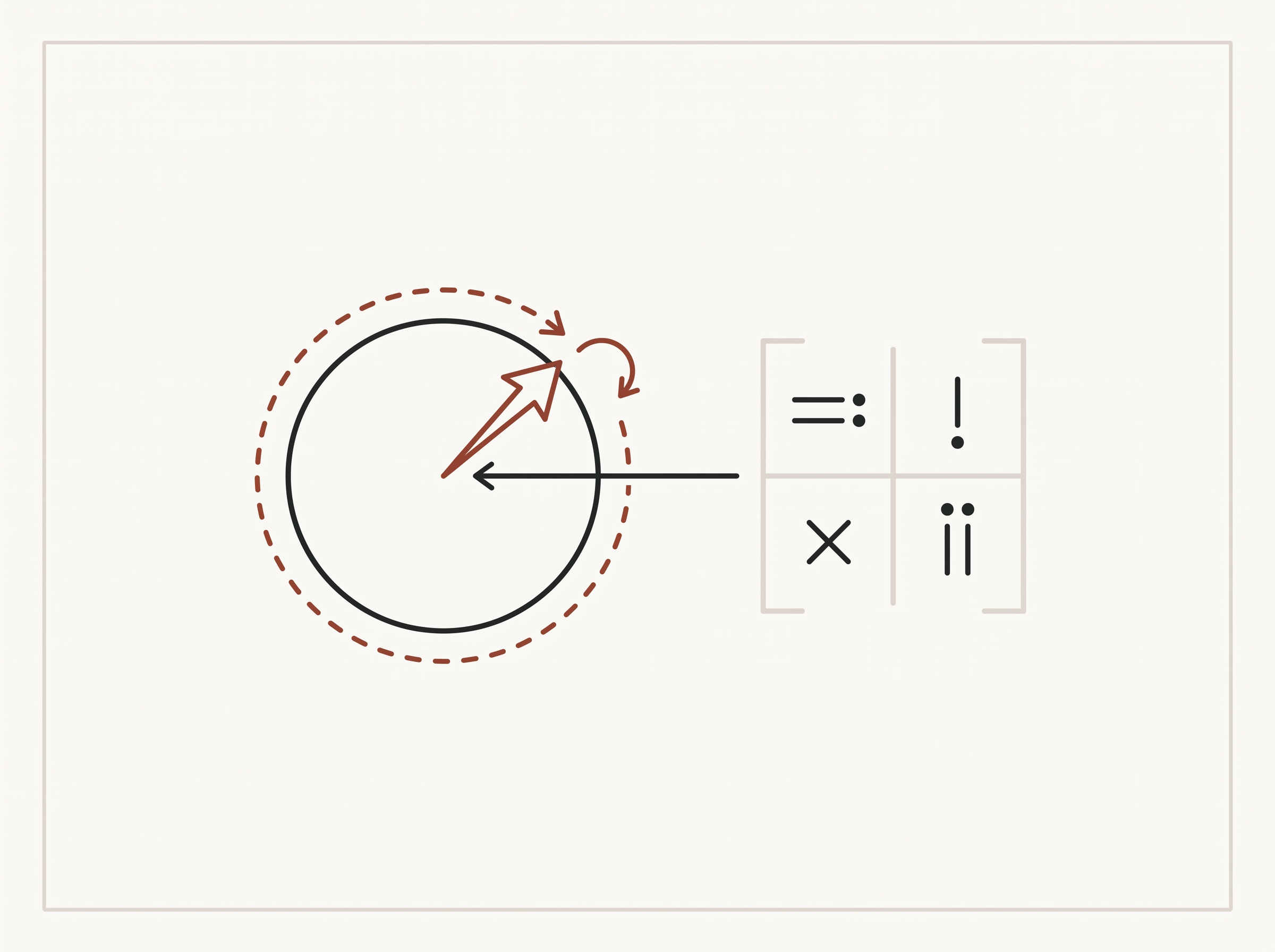
How (and why) to raise e to the power of a matrix, from 3Blue1Brown (Grant Sanderson), published April 1, 2021, 27 minutes. Everything below is written from a full transcript of the video, in this site’s own words.

The operation, stated plainly

$e^M$ does not mean “multiply $e$ by itself $M$ times.” That reading is nonsense, and the lesson says so immediately.

What it actually means is this. For ordinary real numbers there is an infinite polynomial — the Taylor series — that happens to equal $e^x$:

$$e^x = 1 + x + \frac{x^2}{2!} + \frac{x^3}{3!} + \cdots$$

Every operation in that series is something you can also do to a square matrix: you can multiply a square matrix by itself (that’s $M^2$), you can scale each entry by $1/n!$, and you can add matrices entry by entry. So you just feed the matrix into the polynomial:

$$e^{M} = I + M + \frac{M^2}{2!} + \frac{M^3}{3!} + \cdots$$

with $M^0$ defined as the identity matrix $I$.

The distinction worth holding onto: for real numbers that equation is a theorem — something proved. For matrices (and complex numbers, and stranger objects still) it is a definition — a decision about what the notation will mean. Sanderson frames the choice honestly: you can call reusing the $e^{(\cdot)}$ notation a blatant abuse of it, or you can call it a good example of the cycle between discovery and invention in mathematics. Both readings are fair.

The example that shows it isn’t nonsense

Take the matrix

$$M = \begin{bmatrix} 0 & -\pi \ \pi & 0 \end{bmatrix}$$

and run the series. The powers of that matrix cycle with period four (it is a 90° rotation scaled by $\pi$), and when you add up all infinitely many terms, the entries assemble themselves into the Taylor series for sine and cosine. The sum converges to $-I$ — negative one times the identity matrix.

That is Euler’s identity, $e^{i\pi} = -1$, in matrix form. The reason it works: multiplication by $i\pi$ on the complex plane does the same job as multiplication by that matrix — rotate by 90° and scale by $\pi$. Drop the scaling and $J = \begin{bmatrix} 0 & -1 \ 1 & 0 \end{bmatrix}$ is the exact analogue of $i$ alone: a pure 90° rotation, nothing else.

What it’s actually for: differential equations

The reason this operation exists at all is that it solves a whole class of differential equations.

In one dimension, $\frac{dx}{dt} = rx$ has solution $x(t) = e^{rt}x_0$. The lesson makes a point here that is worth stealing for teaching generally: don’t think of $e^{rt}$ as the solution. Think of it as a thing that acts on an initial condition to produce a solution. $e^{rt}$ is only the solution when you happen to start at 1.

Now push it up a dimension. If a vector changes such that its rate of change is a matrix times itself,

$$\frac{d\vec{v}}{dt} = M\vec{v}$$

with $M$ constant in time, then the solution is $\vec{v}(t) = e^{Mt}\vec{v}_0$ — the exponential produces a matrix that changes with time, and it acts on the initial vector. A central reason the definition is worth having is that it makes this statement true.

The proof sketch is short enough to follow in your head: write out the series, differentiate term by term, and the power rule cancels against the factorials so cleanly that what’s left is $M$ times the original expression. So $\frac{d}{dt}e^{Mt}\vec v_0 = M e^{Mt}\vec v_0$, which is the equation you started with. (For a finite square matrix the series converges everywhere, so no rigor is being skipped here — the mechanism of term-by-term differentiation is the point.)

The visualization worth the whole 27 minutes

Draw the vector field: at every point $\vec{v}$ in the space, attach the vector $M\vec{v}$. That picture is the differential equation — it says “if a state is here, this is how fast and which way it’s moving.”

Then $e^{Mt}$ has a completely concrete meaning: let every possible starting point flow along that field for $t$ units of time, and $e^{Mt}$ is the matrix describing where everything ended up. Rotation fields give rotation matrices. Fields that stretch along one diagonal and squeeze along another give matrices that stretch and squeeze, more extremely as $t$ grows.

That reframing is the real payoff. It turns “compute this insane infinite sum” into “look at the flow and read off the answer.”

Where this touches physics — and this site

Schrödinger’s equation is of the form $\partial_t \psi = A\psi$, usually written $i\hbar,\partial_t\psi = H\psi$, so that $A = -iH/\hbar$. When $H$ is Hermitian, as it normally is, $A$ is skew-Hermitian ($A^\dagger = -A$) — the direct analogue of the real skew-symmetric property ($J^\top = -J$) that made $M\vec v$ perpendicular to $\vec v$ in the toy model above. (It is not the property $J^2 = -I$ that made the Euler example work out to a clean rotation; a general Hermitian $H$ doesn’t give you that.) Skew-Hermitian generators are exactly the ones whose flow is unitary: probability is conserved, and in the energy eigenbasis each component picks up nothing but a phase. Superpositions of different energies do more than that — the relative phases between components drive interference, spreading, and everything else a wavefunction actually does. The $i$ is the visible marker of the skew-Hermitian structure, not the cause of it on its own.

One distinction worth being precise about: the “rotation” here is unitary evolution on the state space, not rotation in physical position space. The toy example above literally spins an arrow in a flat plane. A wavefunction $\psi(x)$ doesn’t spin in space the way that arrow does — it acquires phase, interferes, disperses. The two are the same algebra, not the same geometry. (This account also assumes a fixed, time-independent generator, the same assumption the toy differential equation made above — a time-dependent $H(t)$ needs the more general time-ordered exponential.)

The same pattern recurs anywhere you exponentiate a rotation-like generator times time: complex exponentials, quaternions, and a great many of the operators in quantum mechanics.

This connects directly to Erwin Schrödinger and to the general point this site keeps returning to: an equation that looks like an arbitrary formula usually turns out to be describing a motion. Here the motion is unitary evolution in state space, and $i$ is one of the things announcing it.

Catalog status: Proven Systems

Matrix exponentiation is settled mathematics — a definition plus a theorem about what it solves, both provable, neither in dispute. Nothing here is a claim under test.